Bandstructures
The eigenpairs (eigenvalues and eigenvectors) of a Hamiltonian or ParametricHamiltonian at given Bloch phases ϕᵢ can be obtained with spectrum:
julia> h = LP.honeycomb() |> hopping(1); ϕᵢ = (0, π);

julia> eᵢ, ψᵢ = spectrum(h, ϕᵢ; solver = EigenSolvers.LinearAlgebra())
Spectrum{Float64,ComplexF64} :
Energies:
2-element Vector{ComplexF64}:
 -1.0 + 0.0im
  1.0 + 0.0im
States:
2×2 Matrix{ComplexF64}:
  0.707107-8.65956e-17im  0.707107-8.65956e-17im
 -0.707107+0.0im          0.707107+0.0im
The above destructuring syntax assigns eigenvalues and eigenvectors to eᵢ and ψᵢ, respectively. The available eigensolvers and their options can be checked in the EigenSolvers docstrings. They are supported through the extension mechanism in Julia, so they require additional libraries to be loaded first, such as using Arpack or using ArnoldiMethod.
EigenSolvers.Arpack relies on a Fortran library that is not currently thread-safe. If you launch Julia with multiple threads, they will not be used with this specific solver. Otherwise Arpack would segfault.
We define a "bandstructure" of an h::AbstractHamiltonian as a linear interpolation of its eigenpairs over a portion of the Brillouin zone, which is discretized with a base mesh of ϕᵢ values. At each ϕᵢ of the base mesh, the Bloch matrix h(ϕᵢ) is diagonalized with spectrum. The adjacent eigenpairs eⱼ(ϕᵢ), ψⱼ(ϕᵢ) are then connected ("stitched") together into a number of band meshes with vertices (ϕᵢ..., eⱼ(ϕᵢ)) by maximizing the overlap of adjacent ψⱼ(ϕᵢ) (since the bands should be continuuous). Degenerate eigenpairs are collected into a single node of the band mesh.
The bandstructure of an h::AbstractHamiltonian is computed using bands:
julia> ϕ₁points = ϕ₂points = range(0, 2π, length = 19);

julia> b = bands(h, ϕ₁points, ϕ₂points)
Bandstructure{Float64,3,2}: 3D Bandstructure over a 2-dimensional parameter space of type Float64
  Subbands  : 1
  Vertices  : 720
  Edges     : 2016
  Simplices : 1296
  Metadata  : Missing
The first argument is the AbstractHamiltonian. Here it is defined on an L=2 dimensional lattice. The subsequent arguments are collections of Bloch phases on each of the L axes of the Brillouin zone, whose direct product ϕ₁points ⊗ ϕ₂points defines our base mesh of ϕᵢ points. Here it is a uniform 19×19 grid. We can once more use qplot to visualize the bandstructure, or more precisely the band meshes:
julia> using GLMakie; qplot(b)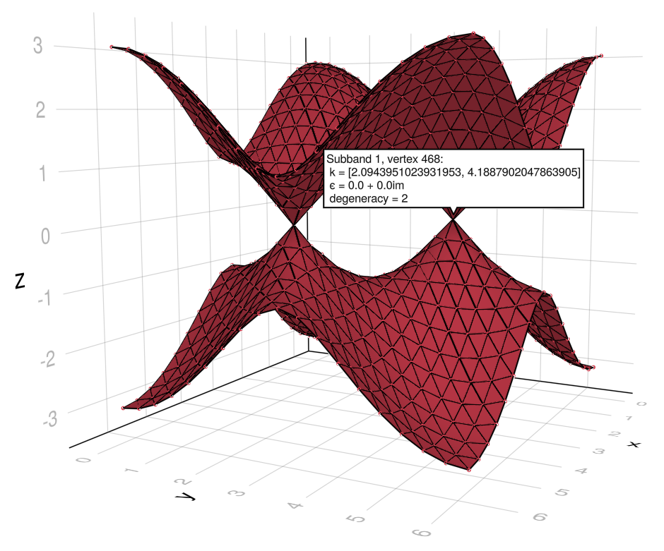
The dots on the bands are the band mesh vertices (ϕᵢ..., eⱼ(ϕᵢ)). They can be omitted with the qplot keyword hide = :nodes (or hide = :vertices, both are equivalent).
Band defects
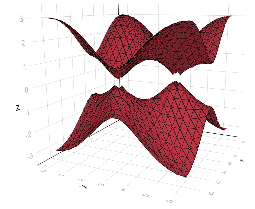
Note that the uniform grid contains the Dirac points. This is the reason for the number 19 of Bloch phases used above. Note also that it is identified as a point in the bands with degeneracy = 2 (the rest have degeneracy = 1). As mentioned, the points on the bands are connected based on eigenstate overlaps between adjacent ϕᵢs. This interpolation algorithm can deal with subspace degeneracies, as here. However, Dirac points (and Diabolical Points in general) must belong to the mesh for the method to work. If the number of points is reduced to 18 per axis, the Dirac points become unavoidable band dislocations, that appear as missing simplices in the bands:
If a Dirac point or other type of band dislocation point happens to not belong to the sampling grid, it can be added with the bands keyword defects. Then, it can be reconnected with the rest of the band by increasing the patches::Integer keyword (see bands docstring for details). This "band repair" functionality is experimental, and should only be necessary in some cases with Diabolical Points.
Coordinate mapping and band linecuts
The direct product of the ϕᵢpoints above define a rectangular mesh over which we want to compute the bandstructure. By default, this mesh is taken as a discretization of Bloch phases, so h(ϕᵢ) is diagonalized at each point of the base mesh. We might want, however, a different relation between the mesh and the parameters passed to h, for example if we wish to use wavevectors k instead of Bloch phases ϕᵢ = k⋅Aᵢ for the mesh. This is achieved with the mapping keyword, which accepts a function mapping = (mesh_points...) -> bloch_phases,
julia> h = LP.honeycomb() |> hopping(2); k₁points = range(-2π, 2π, length = 51); k₂points = range(-2π, 2π, length = 51);

julia> Kpoints = [SA[cos(θ) -sin(θ); sin(θ) cos(θ)] * SA[4π/3,0] for θ in range(0, 5*2π/6, length = 6)];

julia> ϕ(k...) =  SA[k...]' * bravais_matrix(h)
ϕ (generic function with 1 method)

julia> b = bands(h,  k₁points, k₂points; mapping = ϕ, defects = Kpoints, patches = 20);

julia> using GLMakie; qplot(b, hide = (:nodes, :wireframe), color = :orange)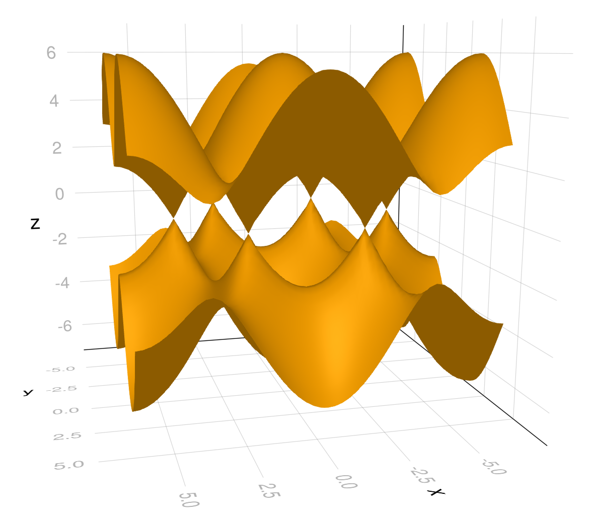
To compute a bandstructure linecut along a polygonal line in the Brillouin zone, we could once more use the mapping functionality, mapping a set of points xᵢ::Real in the mesh to Bloch phases ϕᵢ that defines the nodes of the polygonal path, and interpolating linearly between them. To avoid having to construct this mapping ourselves, mapping accepts a second type of input for this specific usecase, mapping = xᵢ => ϕᵢ. Here, ϕᵢ can be a collection of Tuples, SVector{L}, or even Symbols denoting common names for high-symmetry points in the Brillouin zone, such as :Γ, :K, :K´, :M, :X, :Y, and :Z. The following gives a Γ-K-M-Γ linecut for the bands above, where the (Γ, K, M, Γ) points lie at x = (0, 2, 3, 4), respectively, with 10 subdivisions in each segment,
julia> b = bands(h, subdiv((0, 2, 3, 4), 10); mapping = (0, 2, 3, 4) => (:Γ, :K, :M, :Γ));

julia> qplot(b, axis = (; xticks = ([0, 2, 3, 4], ["Γ", "K", "M", "Γ"]), ylabel = "ϵ"))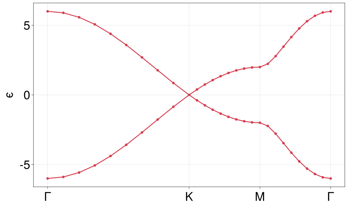
The subdiv function is a convenience function provided by Quantica.jl that generalizes range (see the corresponding docstring for comprehensive details). It is useful to create collections of numbers as subdivisions of intervals, as in the example above. In its simplest form subdiv(min, max, npoints) is is equivalent to range(min, max, npoints).
The mapping keyword understand a third syntax that can be used to map a mesh to the space of Bloch phases and parameters of a ParametricHamiltonian. To this end we use mapping = (mesh_points...) -> ftuple(bloch_phases...; params...). The ftuple function creates a FrankenTuple, which is a hybrid between a Tuple and a NamedTuple. For example, in the following 1D SSH chain we can compute the bandstructure as a function of Bloch phase ϕ and hopping t´, and plot it using more customization options
julia> h = LP.linear() |> supercell(2) |> @hopping((r, dr; t = 1, t´ = 2) -> iseven(r[1]-1/2) ? t : t´);

julia> b = bands(h, subdiv(0, 2π, 11), subdiv(0, 10, 11), mapping = (ϕ, y) -> ftuple(ϕ; t´ = y/5), patches = 20)
Bandstructure{Float64,3,2}: 3D Bandstructure over a 2-dimensional parameter space of type Float64
  Subbands  : 1
  Vertices  : 249
  Edges     : 664
  Simplices : 416
  Metadata  : Missing

julia> qplot(b, nodedarken = 0.5, axis = (; aspect = (1,1,1), perspectiveness = 0.5, xlabel = "ϕ", ylabel = "t´/t", zlabel = "ϵ"), fancyaxis = false)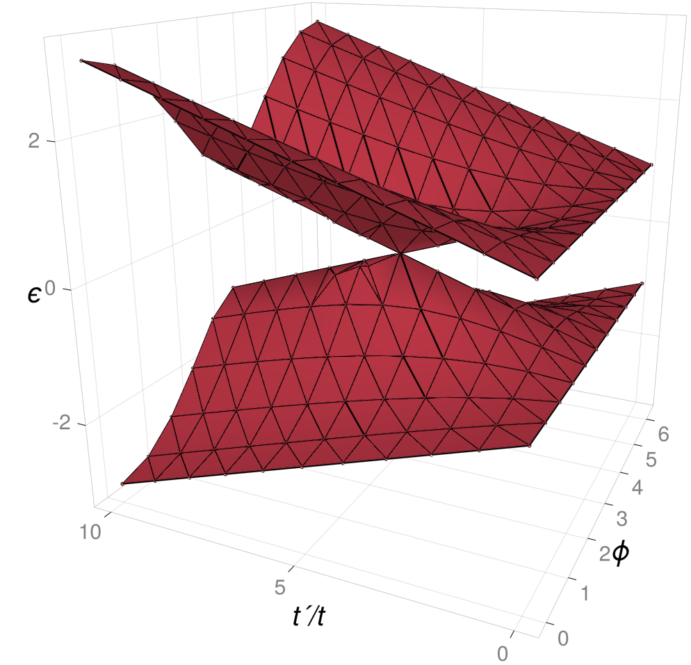
Note that since we didn't specify a value for t, it assumed its default t=1. In this case we needed to patch the defect at (ϕ, t´) = (π, 1) (topological transition) using the patches keyword to avoid a band dislocation.
If no parameters are specified or mapped, they take their default values. For example, this produces the 1D bandstructure of the SSH model for the default t = 1, t´ = 2 over the default 1D mesh (49 points, uniformly distributed in [-π, π])
julia> qplot(bands(h))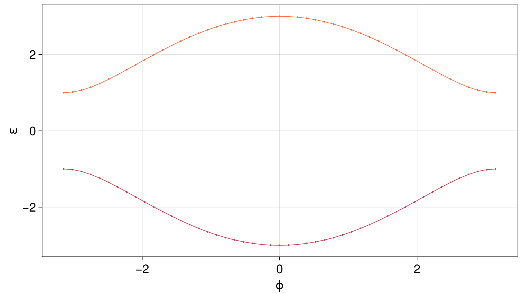
The function Quantica.gaps(h, µ) can be used to efficiently calculate the gaps respect to chemical potential µ at local band minima, but only for 1D Hamiltonian's for the moment. Similarly Quantica.decay_lengths(h, µ; reverse = false) will yield the decay lengths of the evanescent modes of h at energy µ (towards the positive direction, unless reverse = true). Both functions are unexported and experimental.
Band indexing and slicing
The individual subbands in a given b::Bandstructure can be obtained with b[inds] with inds::Integer or inds::Vector, just as if b where a normal AbstractVector. The extracted subbands can also be plotted directly. The following example has 12 subbands, of which we extract and plot the first and last
julia> h = LP.triangular() |> supercell(4) |> hopping(1) + onsite(r -> 4*rand());

julia> b = bands(h, subdiv(0, 2π, 31), subdiv(0, 2π, 31))
Bandstructure{Float64,3,2}: 3D Bandstructure over a 2-dimensional parameter space of type Float64
  Subbands  : 12
  Vertices  : 15376
  Edges     : 44152
  Simplices : 28696
  Metadata  : Missing

julia> qplot(b, hide = (:nodes, :wireframe))

julia> qplot(b[[1, end]], hide = (:nodes, :wireframe))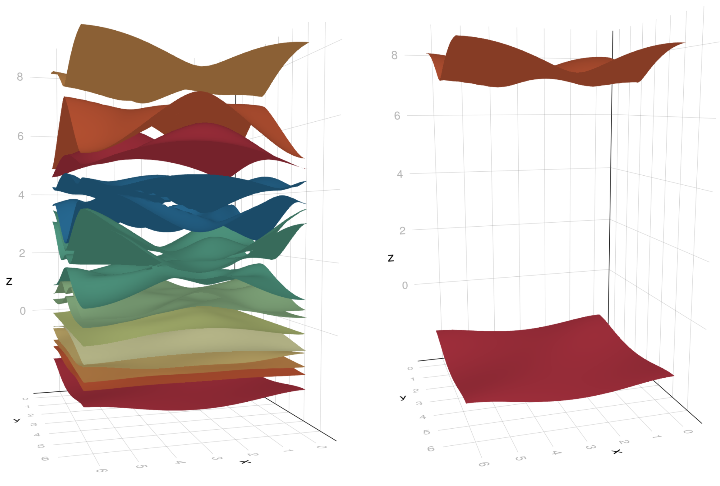
For a band in a 2D Brillouin zone, we can also obtain the intersection of a bandstructure with a plane of constant energy ϵ=2 using the syntax b[(:,:,2)]. A section at fixed Bloch phase ϕ₁=0 (or mesh coordinate x₁=0 if mapping was used), can be obtained with b[(0,:,:)]. This type of band slicing can be generalized to higher dimensional bandstructures, or to more than one constrain (e.g. energy and/or a subset of Bloch phases). As an example, this would be the Fermi surface of a nearest-neighbor cubic-lattice Hamiltonian at Fermi energy µ = 0.2t
julia> pts = subdiv(0, 2π, 41); b = LP.cubic() |> hopping(1) |> bands(pts, pts, pts)
Bandstructure{Float64,4,3}: 4D Bandstructure over a 3-dimensional parameter space of type Float64
  Subbands  : 1
  Vertices  : 68921
  Edges     : 462520
  Simplices : 384000
  Metadata  : Missing

julia> qplot(b[(:, :, :, 0.2)], hide = (:nodes, :wireframe))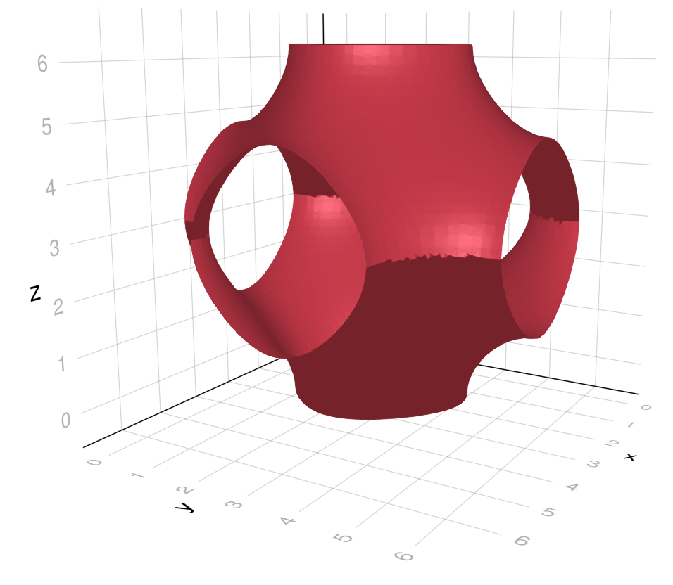
The above example showcases a current (cosmetic) limitation of the band slicing algorithm: it sometimes fails to align all faces of the resulting manifold to the same orientation. The dark and bright regions of the surface above reveals that approximately half of the faces in this case are facing inward and the rest outward.
Band metadata
We can compute metadata associated to each vertex of a bandstructure. This is done with the metadata keyword of bands, which accepts a callable object of a AbstractBandsMetadata subtype. Currently we have m = berry_curvature(h) as a possible metadata object. It computes the (Abelian or non-Abelian) Berry curvature of the subbands of a 2D h::AbstractHamiltonian at given Bloch phases φs with m(φs [, subband_indices]). The following example computes the Abelian Berry curvature of a gapped graphene model and colors the bands accordingly
julia> h = LP.honeycomb() |> onsite(0.5, sublats = :A) - onsite(0.5, sublats = :B) + hopping(1)
Hamiltonian{Float64,2,2}: Hamiltonian on a 2D Lattice in 2D space
  Bloch harmonics  : 5
  Harmonic size    : 2 × 2
  Orbitals         : [1, 1]
  Element type     : scalar (ComplexF64)
  Onsites          : 2
  Hoppings         : 6
  Coordination     : 3.0

julia> m = berry_curvature(h)
BerryCurvature: Abelian Berry curvature of a 2D AbstractHamiltonian

julia> m(SA[2π/3,4π/3])
2-element Vector{Float64}:
  68.37862509316868
 -68.37862509316868

julia> b = bands(h; metadata = m)  # here `h` needs to be a 2D non-parametric Hamiltonian.
Bandstructure{Float64,3,2}: 3D Bandstructure over a 2-dimensional parameter space of type Float64
  Subbands  : 2
  Vertices  : 4802
  Edges     : 14016
  Simplices : 9216
  Metadata  : Float64

julia> qplot(b, color = (ψ,ϵ,k,m) -> m, hide = :wireframe, size = 0, colormap = :balance)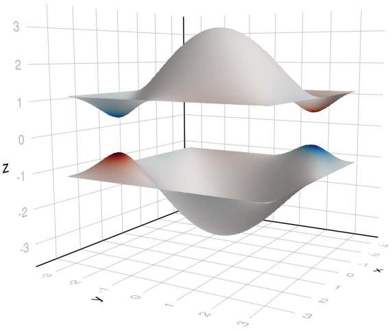
The berry_curvature metadata generator can also compute the non-Abelian Berry curvature of at most d-degenerate subspaces with the syntax bc = berry_curvature(h; maxdim = d). The non-Abelian Berry curvature of states with indices in rng::UnitRange are computed with bc(φs, rng). This returns a Matrix of size length(rng)×length(rng). This requires length(rng)<=d.