Observables
We are almost at our destination now. We have defined a Lattice, a Model for our system, we applied the Model to the Lattice to obtain a Hamiltonian or a ParametricHamiltonian, and finally, after possibly attaching some contacts to outside reservoirs and specifying a GreenSolver, we obtained a GreenFunction. It is now time to use the GreenFunction to obtain some observables of interest.
Currently, we have the following observables built into Quantica.jl (with more to come in the future)
ldos: computes the local density of states at specific energy and sitesdensitymatrix: computes the density matrix at thermal equilibrium on specific sites.current: computes the local current density along specific directions, and at specific energy and sitestransmission: computes the total transmission between contactsconductance: computes the differential conductancedIᵢ/dVⱼbetween contactsiandjjosephson: computes the supercurrent and the current-phase relation through a given contact in a superconducting system
See the corresponding docstrings for full usage instructions. Here we will present some basic examples
Local density of states (LDOS)
Let us compute the LDOS in a cavity like in the previous section. Instead of computing the Green function between a contact to an arbitrary point, we can construct an object d = ldos(g(ω)) without any contacts. By using a small imaginary part in ω, we broaden the discrete spectrum, and obtain a finite LDOS. Then, we can pass d directly as a site shader to qplot
julia> h = LP.square() |> onsite(4) - hopping(1) |> supercell(region = r -> norm(r) < 40*(1+0.2*cos(5*atan(r[2],r[1]))));

julia> g = h |> greenfunction;

julia> d = ldos(g(0.1 + 0.001im))
LocalSpectralDensitySolution{Float64} : local density of states at fixed energy and arbitrary location
  kernel   : LinearAlgebra.UniformScaling{Bool}(true)

julia> qplot(h, hide = :hops, sitecolor = d, siteradius = d, minmaxsiteradius = (0, 2), sitecolormap = :balance)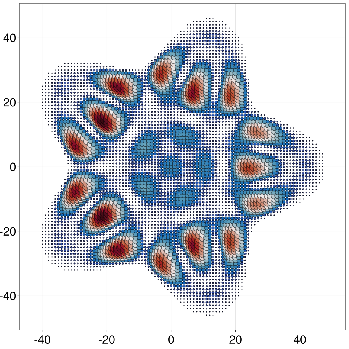
Note that d[sites...] produces a vector with the LDOS at sites defined by siteselector(; sites...) (d[] is the ldos over all sites). We can also define a kernel to be traced over orbitals to obtain the spectral density of site-local observables (see diagonal slicing in the preceding section).
Density matrix
We can also compute the convolution of the density of states with the Fermi distribution f(ω)=1/(exp((ω-μ)/kBT) + 1), which yields the density matrix in thermal equilibrium, at a given temperature kBT and chemical potential μ. This is computed with ρ = densitymatrix(gs, (ωmin, ωmax)). Here gs = g[sites...] is a GreenSlice, and (ωmin, ωmax) are integration bounds (they should span the full bandwidth of the system). Then, ρ(µ, kBT = 0; params...) will yield a matrix over the selected sites for a set of model params.
julia> ρ = densitymatrix(g[region = RP.circle(1)], (-0.1, 8.1))
DensityMatrix{DensityMatrixIntegratorSolver}: density matrix on specified sites

julia> @time ρ(4)
  4.594645 seconds (111.82 k allocations: 4.890 GiB, 2.81% gc time, 0.86% compilation time)
5×5 OrbitalSliceMatrix{ComplexF64,Array}:
          0.5+0.0im          -7.35075e-10+3.40256e-15im  0.204478+4.46023e-14im  -7.35077e-10-1.13342e-15im  -5.70426e-10-2.22213e-15im
 -7.35075e-10-3.40256e-15im           0.5+0.0im          0.200693-4.46528e-14im  -5.70431e-10+3.53853e-15im  -7.35092e-10-4.07992e-16im
     0.204478-4.46023e-14im      0.200693+4.46528e-14im       0.5+0.0im              0.200693+6.7793e-14im       0.204779-6.78156e-14im
 -7.35077e-10+1.13342e-15im  -5.70431e-10-3.53853e-15im  0.200693-6.7793e-14im            0.5+0.0im            -7.351e-10+2.04708e-15im
 -5.70426e-10+2.22213e-15im  -7.35092e-10+4.07992e-16im  0.204779+6.78156e-14im    -7.351e-10-2.04708e-15im           0.5+0.0im
Note that the diagonal is 0.5, indicating half-filling.
The default algorithm used here is slow, as it relies on numerical integration in the complex plane. Some GreenSolvers have more efficient implementations. If they exist, they can be accessed by omitting the (ωmin, ωmax) argument. For example, using GS.Spectrum:
julia> @time g = h |> greenfunction(GS.Spectrum());
 18.249136 seconds (75 allocations: 1.567 GiB, 0.67% gc time)

julia> ρ = densitymatrix(g[region = RP.circle(1)])
DensityMatrix{DensityMatrixSpectrumSolver}: density matrix on specified sites

julia> @time ρ(4)  # second-run timing
  0.029662 seconds (7 allocations: 688 bytes)
5×5 OrbitalSliceMatrix{ComplexF64,Array}:
         0.5+0.0im   -6.6187e-16+0.0im  0.204478+0.0im   2.49658e-15+0.0im  -2.6846e-16+0.0im
 -6.6187e-16+0.0im           0.5+0.0im  0.200693+0.0im  -2.01174e-15+0.0im   1.2853e-15+0.0im
    0.204478+0.0im      0.200693+0.0im       0.5+0.0im      0.200693+0.0im     0.204779+0.0im
 2.49658e-15+0.0im  -2.01174e-15+0.0im  0.200693+0.0im           0.5+0.0im  1.58804e-15+0.0im
 -2.6846e-16+0.0im    1.2853e-15+0.0im  0.204779+0.0im   1.58804e-15+0.0im          0.5+0.0im
Note, however, that the computation of g is much slower in this case, due to the need of a full diagonalization. A better algorithm choice in this case is GS.KPM. It requires, however, that we define the region for the density matrix beforehand, as a nothing contact.
julia> @time g = h |> attach(nothing, region = RP.circle(1)) |> greenfunction(GS.KPM(order = 10000, bandrange = (0,8)));
Computing moments: 100%|███████████████████████████████████████████████████████████████████████████████████████| Time: 0:00:01
  1.360412 seconds (51.17 k allocations: 11.710 MiB)

julia> ρ = densitymatrix(g[1])
DensityMatrix{DensityMatrixKPMSolver}: density matrix on specified sites

julia> @time ρ(4)
  0.004024 seconds (3 allocations: 688 bytes)
5×5 OrbitalSliceMatrix{ComplexF64,Array}:
         0.5+0.0im  2.15097e-17+0.0im   0.20456+0.0im  2.15097e-17+0.0im   3.9251e-17+0.0im
 2.15097e-17+0.0im          0.5+0.0im  0.200631+0.0im  1.05873e-16+0.0im  1.70531e-18+0.0im
     0.20456+0.0im     0.200631+0.0im       0.5+0.0im     0.200631+0.0im      0.20482+0.0im
 2.15097e-17+0.0im  1.05873e-16+0.0im  0.200631+0.0im          0.5+0.0im  1.70531e-18+0.0im
3.9251e-17+0.0im 1.70531e-18+0.0im 0.20482+0.0im 1.70531e-18+0.0im 0.5+0.0imThe integration algorithm allows many different integration paths that can be adjusted to each problem, see the Paths docstring. Another versatile choice is Paths.radial(ωrate, ϕ). This one is called with ϕ = π/4 when doing ρ = densitymatrix(gs::GreenSlice, ωrate::Number). In the example above this is slightly faster than the (ωmin, ωmax) choice, which resorts to Paths.sawtooth(ωmin, ωmax).
Current
A similar computation can be done to obtain the current density, using J = current(g(ω), direction = missing). This time J[sᵢ, sⱼ] yields a sparse matrix of current densities along a given direction for each hopping (or the current norm if direction = missing). Passing J as a hopping shader yields the equilibrium current in a system. In the above example we can add a magnetic flux to make this current finite
julia> h = LP.square() |> supercell(region = r -> norm(r) < 40*(1+0.2*cos(5*atan(r[2],r[1])))) |> onsite(4) - @hopping((r, dr; B = 0.1) -> cis(B * dr[1] * r[2]));

julia> g = h |> greenfunction;

julia> J = current(g(0.1; B = 0.01))
CurrentDensitySolution{Float64} : current density at a fixed energy and arbitrary location
  charge      : LinearAlgebra.UniformScaling{Int64}(-1)
  direction   : missing

julia> qplot(h, siteradius = 0.08, sitecolor = :black, siteoutline = 0, hopradius = J, hopcolor = J, minmaxhopradius = (0, 2), hopcolormap = :balance, hopdarken = 0)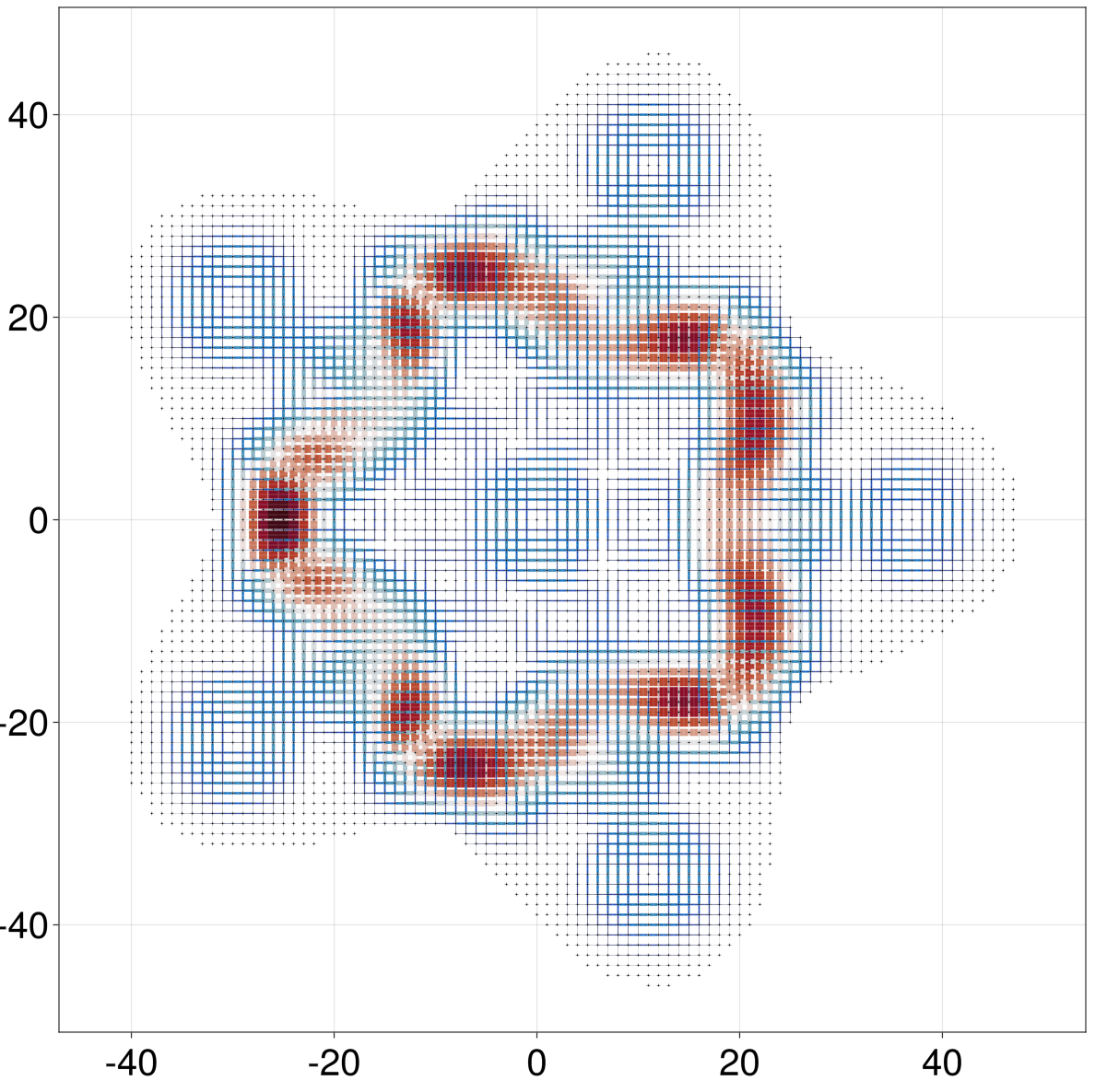
Note that we built the supercell before applying the model with the magnetic flux. Not doing so would make the gauge field be repeated in each unit cell when expanding the supercell. This was mentioned in the section on Hamiltonians, and is a common mistake when modeling systems with position dependent fields.
Transmission
The transmission Tᵢⱼ from contact j to contact i can be computed using transmission. This function accepts a GreenSlice between the contact. Let us recover the four-terminal setup of the preceding section, but let's make it bigger this time
julia> hcentral = LP.square() |> hopping(-1) |> supercell(region = RP.circle(100) | RP.rectangle((202, 50)) | RP.rectangle((50, 202)))

julia> glead = LP.square() |> hopping(-1) |> supercell((1, 0), region = r -> abs(r[2]) <= 50/2) |> greenfunction(GS.Schur(boundary = 0));

julia> Rot = r -> SA[0 -1; 1 0] * r;  # 90º rotation function

julia> g = hcentral |>
           attach(glead, region = r -> r[1] ==  101) |>
           attach(glead, region = r -> r[1] == -101, reverse = true) |>
           attach(glead, region = r -> r[2] ==  101, transform = Rot) |>
           attach(glead, region = r -> r[2] == -101, reverse = true, transform = Rot) |>
           greenfunction;

julia> gx1 = abs2.(g(-3.96)[siteselector(), 1]);

julia> qplot(hcentral, hide = :hops, siteoutline = 1, sitecolor = gx1, siteradius = gx1, minmaxsiteradius = (0, 2), sitecolormap = :balance)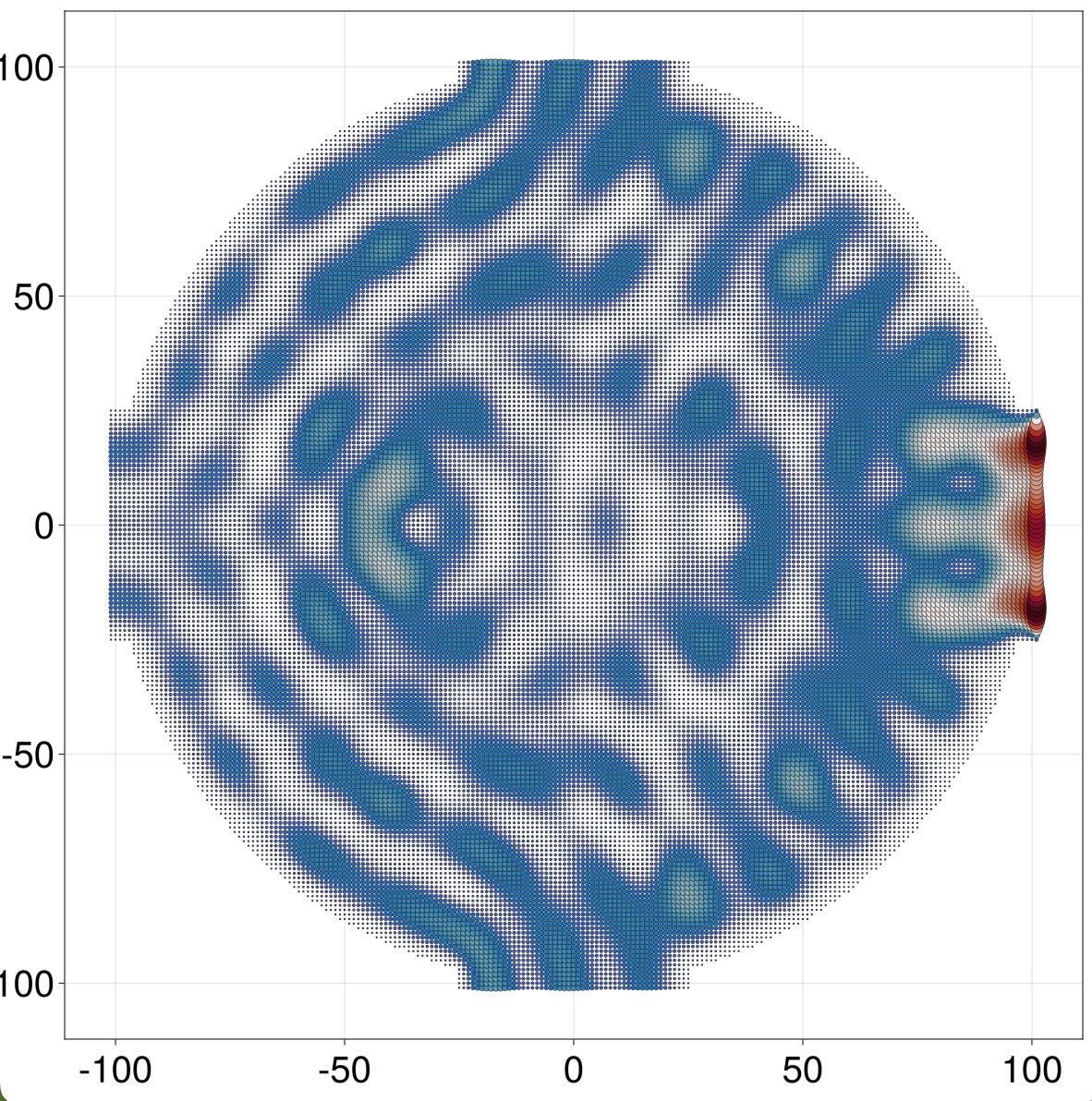
In the above example gx1 is a matrix with one row per orbital in hcentral. The color and radii of each site is obtained from the sum of each row. If gx1 were a vector, the color/radius of site i would be taken as gx1[i]. See plotlattice for more details and other shader types.
It's apparent from the plot that the transmission from right to left (T₂₁ here) at this energy of 0.04 is larger than from right to top (T₃₁). Is this true in general? Let us compute the two transmissions as a function of energy. To show the progress of the calculation we can use a monitor package, such as ProgressMeter
julia> using ProgressMeter

julia> T₂₁ = transmission(g[2,1]); T₃₁ = transmission(g[3,1]); ωs = subdiv(-4, 4, 201);

julia> T₂₁ω = @showprogress [T₂₁(ω) for ω in ωs]; T₃₁ω = @showprogress [T₃₁(ω) for ω in ωs];
Progress: 100%|██████████████████████████████████████████████████████████████| Time: 0:01:02
Progress: 100%|██████████████████████████████████████████████████████████████| Time: 0:01:00

julia> f = Figure(); a = Axis(f[1,1], xlabel = "ω/t", ylabel = "T(ω)"); lines!(a, ωs, T₂₁ω, label = L"T_{2,1}"); lines!(a, ωs, T₃₁ω, label = L"T_{3,1}"); axislegend("Transmission", position = :lt); f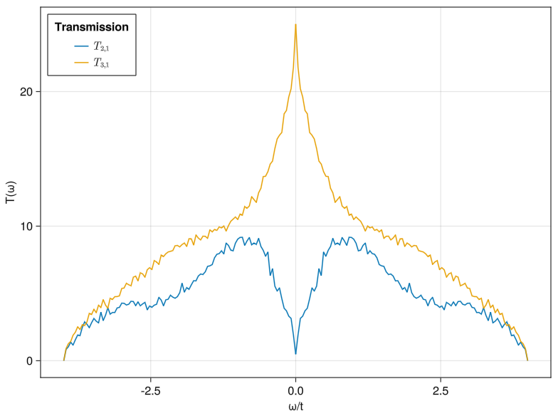
So we indeed find that the 90-degree transmission T₃₁ is indeed larger than the forward transmission T₂₁ for all energies. The rapid oscillations are due to mesoscopic fluctuations.
Note that transmission gives the total transmission, which is the sum of the transmission probability from each orbital in the source contact to any other orbital in the drain contact. As such it is not normalized to 1, but to the number of source orbitals. It also gives the local conductance from a given contact in units of $e^2/h$ according to the Landauer formula, $G_j = e^2/h \sum_i T_{ij}(eV)$.
Conductance
Local and non-local differential conductance $G_{ij} = dI_i/dV_j$ can be computed with G = conductance(g[i,j]). Calling G(ω) returns the conductance at bias $eV = \omega$ in units of $e^2/h$. Let's look at the local differential conductance into the right contact in the previous example
julia> G₁₁ = conductance(g[1,1])
Conductance{Float64}: Zero-temperature conductance dIᵢ/dVⱼ from contacts i,j, in units of e^2/h
  Current contact  : 1
  Bias contact     : 1

julia> ωs = subdiv(-4, 4, 201); Gω = @showprogress [G₁₁(ω) for ω in ωs];
Progress: 100%|██████████████████████████████████████████████████████████████| Time: 0:01:01

julia> f = Figure(); a = Axis(f[1,1], xlabel = "eV/t", ylabel = "G [e²/h]"); lines!(a, ωs, Gω); f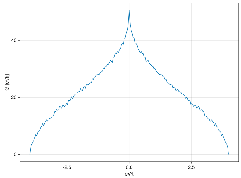
If you compute a non-local conductance such as conductance(g[2,1])(ω) in this example you will note it is negative. This is actually expected. It means that the current flowing into the system through the right contact when you increase the bias in a different contact is negative, because the current is actually flowing out into the right reservoir.
The conductance can also be computed for hybrid (normal-superconducting) systems. To do so, one first needs to write the model in the Nambu representation, i.e. with particle and hole orbitals on each site (first particles, then holes). In the above examples amounts to switching hopping(-1) to hamiltonian(onsite(Δ*σx) - hopping(σz), orbitals = 2), with σx = SA[0 1; 1 0], σz = SA[1 0; 0 -1] and Δ the pairing amplitude. Then we must specify G₁₁ = conductance(g[1,1], nambu = true) to take into account Andreev reflections. The above example with left, bottom and top leads superconducting (with Δ=0.3) yields the following conductance G₁₁ in the right (normal) lead (we leave the implementation as an exercise for the reader).
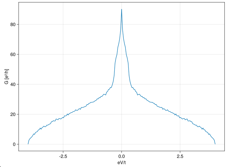
Note that within the gap Andreev reflection leads to an enhancement of conductance, since the contacts are transparent
Josephson
The above example showcases normal-superconductor (NS) conductance, which is a Fermi-surface process in response to an electric bias on the normal contacts. In contrast, supercorconductor-superconductor junctions, also known as Josephson junctions, can exhibit supercurrents carried by the full Fermi sea even without a bias. Usually, this supercurrent flows in response to a phase bias between the superconductors, where by phase we mean the complex phase of the Δ order parameter.
We can compute the supercurrent or the full current-phase relation of a Josephson junction with the command josephson(gs::GreenSlice, ωmax), where gs = g[contact_id] and ωmax is the full bandwidth of the system (i.e. the maximum energy, in absolute value, spanned by the Fermi sea). This latter quantity can be an estimate or even an upper bound, as it is just used to know up to which energy we should integrate the supercurrent. Let us see an example.
julia> σz = SA[1 0; 0 -1];

julia> central_region = RP.circle(50) & !RP.circle(40) | RP.rectangle((4, 10), (-50, 0)) | RP.rectangle((4, 10), (50, 0));

julia> h = LP.square() |> hamiltonian(hopping(-σz), orbitals = 2) |> supercell(region = central_region)

julia> Σ(ω, Δ) = SA[-ω Δ; conj(Δ) -ω]/sqrt(abs2(Δ)-ω^2)

julia> g = h |>
    attach(@onsite((ω; Δ = 0.2) -> Σ(ω, Δ)); region = r -> r[1] < -51) |>
    attach(@onsite((ω; Δ = 0.2, phase = 0) -> Σ(ω, Δ*cis(phase))); region = r -> r[1] > 51) |>
    greenfunction
GreenFunction{Float64,2,0}: Green function of a Hamiltonian{Float64,2,0}
  Solver          : AppliedSparseLUGreenSolver
  Contacts        : 2
  Contact solvers : (SelfEnergyModelSolver, SelfEnergyModelSolver)
  Contact sizes   : (11, 11)
  Hamiltonian{Float64,2,0}: Hamiltonian on a 0D Lattice in 2D space
    Bloch harmonics  : 1
    Harmonic size    : 2884 × 2884
    Orbitals         : [2]
    Element type     : 2 × 2 blocks (ComplexF64)
    Onsites          : 0
    Hoppings         : 10800
    Coordination     : 3.7448

julia> J = josephson(g[1], 4.1)
Josephson{JosephsonIntegratorSolver}: equilibrium Josephson current at a specific contact

julia> qplot(g, children = (; sitecolor = :blue))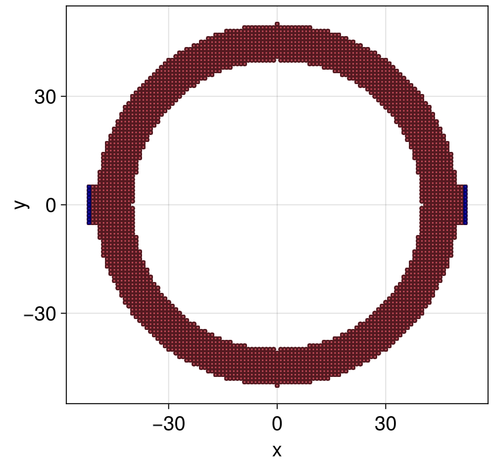
In this case we have chosen to introduce the superconducting leads with a model self-energy, corresponding to a BCS bulk, but any other self-energy form could be used. We have introduced the phase difference (phase) as a model parameter. We can now evaluate the zero-temperature Josephson current simply with
julia> J(phase = 0)
9.006494320662131e-15

julia> J(phase = 0.2)
0.0136818423316157
Note that finite temperatures can be taken using the kBT keyword argument for josephson, see docstring for details.
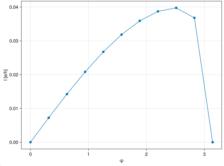
One is often interested in the critical current, which is the maximum of the Josephson current over all phase differences. Quantica.jl can compute the integral over a collection of phase differences simultaneously, which is more efficient that computing them one by one. This is done with
julia> φs = subdiv(0, pi, 11); J = josephson(g[1], 4.1; phases = φs)
Josephson{JosephsonIntegratorSolver}: equilibrium Josephson current at a specific contact

julia> Iφ = J()
11-element Vector{Float64}:
 2.1155016011631047e-14
 0.02145885179546492
 0.042582378252413726
 0.0629936490311923
 0.08222057730191891
 0.09961314919103786
 0.11419800148332125
 0.12437368029947522
 0.12696035667191413
 0.11220061393370946
 4.905386208701179e-11

julia> f = Figure(); a = Axis(f[1,1], xlabel = "φ", ylabel = "I [e/h]"); lines!(a, φs, Iφ); scatter!(a, φs, Iφ); f