GreenFunctions
Up to now we have seen how to define Lattices, Models, Hamiltonians and Bandstructures. Most problems require the computation of different physical observables for these objects, e.g. the local density of states or various transport coefficients. We reduce this general problem to the computation of the retarded Green function
$G^r_{ij}(\omega) = \langle i|(\omega-H-\Sigma(\omega))^{-1}|j\rangle$
where i, j are orbitals, H is the (possibly infinite) Hamiltonian matrix, and Σ(ω) is the self-energy coming from any coupling to other systems (typically described by their own AbstractHamiltonian).
We split the problem of computing Gʳᵢⱼ(ω) of a given h::AbstractHamiltonian into four steps:
- Attach self-energies to
husing the commandoh = attach(h, args...). This produces a new objectoh::OpenHamiltonianwith a number ofContacts, numbered1toN - Use
g = greenfunction(oh, solver)to build ag::GreenFunctionrepresentingGʳ(at arbitraryωandi,j), whereoh::OpenHamiltonianandsolver::AbstractGreenSolver(seeGreenSolversbelow for available solvers) - Evaluate
gω = g(ω; params...)at fixed energyωand model parameters, which produces agω::GreenSolution - Slice
gω[sᵢ, sⱼ]orgω[sᵢ] == gω[sᵢ, sᵢ]to obtainGʳᵢⱼ(ω)as a flat matrix, wheresᵢ, sⱼare either site selectors over sites spanning orbitalsi,j, integers denoting contacts,1toN, or:denoting all contacts merged together.
The two last steps can be interchanged, by first obtaining a gs::GreenSlice with gs = g[sᵢ, sⱼ] and then obtaining the Gʳᵢⱼ(ω) matrix with gs(ω; params...).
A simple example
Here is a simple example of the Green function of a 1D lead with two sites per unit cell, a boundary at cell = 0, and with no attached self-energies for simplicity
julia> hlead = LP.square() |> supercell((1,0), region = r -> 0 <= r[2] < 2) |> hopping(1);

julia> glead = greenfunction(hlead, GreenSolvers.Schur(boundary = 0))
GreenFunction{Float64,2,1}: Green function of a Hamiltonian{Float64,2,1}
  Solver          : AppliedSchurGreenSolver
  Contacts        : 0
  Contact solvers : ()
  Contact sizes   : ()
  Hamiltonian{Float64,2,1}: Hamiltonian on a 1D Lattice in 2D space
    Bloch harmonics  : 3
    Harmonic size    : 2 × 2
    Orbitals         : [1]
    Element type     : scalar (ComplexF64)
    Onsites          : 0
    Hoppings         : 6
    Coordination     : 3.0

julia> gω = glead(0.2)  # we first fix energy to ω = 0.2
GreenSolution{Float64,2,1}: Green function at arbitrary positions, but at a fixed energy

julia> gω[cells = 1:2]  # we now ask for the Green function between orbitals in the first two unit cells to the righht of the boundary
4×4 Matrix{ComplexF64}:
   0.1-0.858258im    -0.5-0.0582576im  -0.48-0.113394im   -0.2+0.846606im
  -0.5-0.0582576im    0.1-0.858258im    -0.2+0.846606im  -0.48-0.113394im
 -0.48-0.113394im    -0.2+0.846606im   0.104-0.869285im   0.44+0.282715im
  -0.2+0.846606im   -0.48-0.113394im    0.44+0.282715im  0.104-0.869285im
Note that the result is a 4 x 4 matrix, because there are 2 orbitals (one per site) in each of the two unit cells. Note also that the GreenSolvers.Schur used here allows us to compute the Green function between distant cells with little overhead
julia> @time gω[cells = 1:2];
  0.000067 seconds (70 allocations: 6.844 KiB)

julia> @time gω[cells = (SA[10], SA[100000])];
  0.000098 seconds (229 allocations: 26.891 KiB)
GreenSolvers
The currently implemented GreenSolvers (abbreviated as GS) are the following
GS.SparseLU()For bounded (
L == 0) AbstractHamiltonians. Default forL == 0.Uses a sparse
LUfactorization to compute the inverse of⟨i|ω - H - Σ(ω)|j⟩, whereΣ(ω)is the self-energy from the contacts.
GS.Spectrum(; spectrum_kw...)For bounded (
L == 0) AbstractHamiltonians.Uses a diagonalization of
H, obtained withspectrum(H; spectrum_kw...), to compute theG⁰ᵢⱼusing the Lehmann representation∑ₖ⟨i|ϕₖ⟩⟨ϕₖ|j⟩/(ω - ϵₖ). Any eigensolver supported byspectrumcan be used here. If there are contacts, it dressesG⁰using a T-matrix approach,G = G⁰ + G⁰TG⁰.
GS.KPM(order = 100, bandrange = missing, kernel = I)For bounded (
L == 0) Hamiltonians, and restricted to sites belonging to contacts (see the section on Contacts).It precomputes the Chebyshev momenta, and incorporates the contact self energy with a T-matrix approach.
GS.Schur(boundary = In, axis = 1, integrate_options...)For 1D (
L == 1) and 2D (L == 2) AbstractHamiltonians with only nearest-cell coupling alongaxis. Default forL=1.Uses a deflating Generalized Schur (QZ) factorization of the generalized eigenvalue 1D problem along
axisto compute the unit-cell self energies. The Dyson equation then yields the Green function between arbitrary unit cells, which is further dressed using a T-matrix approach if the lead has any attached self-energy. Wavevector along transverse axes in 2D systes are numerically integrated with the QuadGK package usingintegrate_options.GS.Bands(bandsargs...; boundary = missing, bandskw...)For unbounded (
L > 0) Hamiltonians.It precomputes a bandstructure
b = bands(h, bandsargs...; kw..., split = false)and then uses analytic expressions for the contribution of each subband simplex to theGreenSolution. Ifboundary = dir => cell_pos, it takes into account the reflections on an infinite boundary perpendicular to Bravais vector numberdir, so that all sites with cell indexc[dir] <= cell_posare removed. Contacts are incorporated using a T-matrix approach. Note that this method, while quite general, is approximate, as it uses linear interpolation of bands within each simplex, so it may suffer from precision issues.To retrieve the bands from a
g::GreenFunctionthat used theGS.Bandssolver, we may usebands(g).
Attaching Contacts
A self energy Σ(ω) acting of a finite set of sites of h (i.e. on a LatticeSlice of lat = lattice(h)) can be incorporated using the attach command. This defines a new Contact in h. The general syntax is oh = attach(h, args...; sites...), where the sites directives define the Contact LatticeSlice (lat[siteselector(; sites...)]), and args can take a number of forms.
The supported attach forms are the following
Generic self-energy
attach(h, gs::GreenSlice, coupling::AbstractModel; sites...)This is the generic form of
attach, which couples some sitesiof ag::Greenfunction(defined by the slicegs = g[i]), tositesofhusing acouplingmodel. This results in a self-energyΣ(ω) = V´⋅gs(ω)⋅Vonhsites, whereVandV´are couplings matrices given bycoupling.Note: currently,
attachof aGreenSlicecreated with direct site indexing (e.g.gs = g[sites(3)]) is not supported. Use asiteselectorinstead, such asgs = g[cells = 1].
Dummy self-energy
attach(h, nothing; sites...)This form merely defines a new contact on the specified
sites, but adds no actual self-energy to it. It is meant as a way to refer to some sites of interest using theg[i::Integer]slicing syntax forGreenFunctions, whereiis the contact index.
Model self-energy
attach(h, model::AbstractModel; sites...)This form defines a self-energy
Σᵢⱼ(ω)in terms ofmodel, which must be composed purely of parametric terms (@onsiteand@hopping) that haveωas first argument, as in e.g.@onsite((ω, r) -> Σᵢᵢ(ω, r))or@hopping((ω, r, dr) -> Σᵢⱼ(ω, r, dr)). This is a modellistic approach, wherein the self-energy is not computed from the properties of anotherAbstractHamiltonian, but rather has an arbitrary form defined by the user.
Matched lead self-energy
attach(h, glead::GreenFunction; reverse = false, transform = identity, sites...)Here
gleadis a GreenFunction of a 1D lead, possibly with a boundary.With this syntax
sitesmust select a number of sites inhwhose position match (after applyingtransformto them and modulo an arbitrary displacement) the sites in the unit cell ofglead. Then, the coupling between these and the first unit cell ofgleadon the positive side of the boundary will be the same as betweengleadunitcells, i.e.V = hlead[(1,)], wherehlead = hamiltonian(glead).If
reverse == true, the lead is reversed before being attached, so that h is coupled throughV = hlead[(-1,)]to the first unitcell on the negative side of the boundary. If there is no boundary, thecell = 0unitcell of thegleadis used.
Generic lead self-energy
attach(h, glead::GreenFunction, model::AbstractModel; reverse = false, transform = identity, sites...)The same as above, but without any restriction on
sites. The coupling between these and the first unit cell ofglead(transformed bytransform) is constructed usingmodel::TightbindingModel. The "first unit cell" is defined as above.
A more advanced example
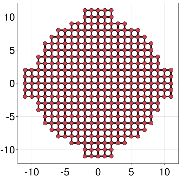
Let us define the classical example of a multiterminal mesoscopic junction. We choose a square lattice, and a circular central region of radius 10, with four leads of width 5 coupled to it at right angles.
We first define a single lead Greenfunction and the central Hamiltonian
julia> glead = LP.square() |> onsite(4) - hopping(1) |> supercell((1, 0), region = r -> abs(r[2]) <= 5/2) |> greenfunction(GS.Schur(boundary = 0));

julia> hcentral = LP.square() |> onsite(4) - hopping(1) |> supercell(region = RP.circle(10) | RP.rectangle((22, 5)) | RP.rectangle((5, 22)));
The two rectangles overlayed on the circle above create the stubs where the leads will be attached:
We now attach glead four times using the Matched lead syntax
julia> Rot = r -> SA[0 -1; 1 0] * r;  # 90º rotation function

julia> g = hcentral |>
    attach(glead, region = r -> r[1] ==  11) |>
    attach(glead, region = r -> r[1] == -11, reverse = true) |>
    attach(glead, region = r -> r[2] ==  11, transform = Rot) |>
    attach(glead, region = r -> r[2] == -11, reverse = true, transform = Rot) |>
    greenfunction
GreenFunction{Float64,2,0}: Green function of a Hamiltonian{Float64,2,0}
  Solver          : AppliedSparseLUGreenSolver
  Contacts        : 4
  Contact solvers : (SelfEnergySchurSolver, SelfEnergySchurSolver, SelfEnergySchurSolver, SelfEnergySchurSolver)
  Contact sizes   : (5, 5, 5, 5)
  Hamiltonian{Float64,2,0}: Hamiltonian on a 0D Lattice in 2D space
    Bloch harmonics  : 1
    Harmonic size    : 353 × 353
    Orbitals         : [1]
    Element type     : scalar (ComplexF64)
    Onsites          : 0
    Hoppings         : 1320
    Coordination     : 3.73938

julia> qplot(g, children = (; selector = siteselector(; cells = 1:5), sitecolor = :blue))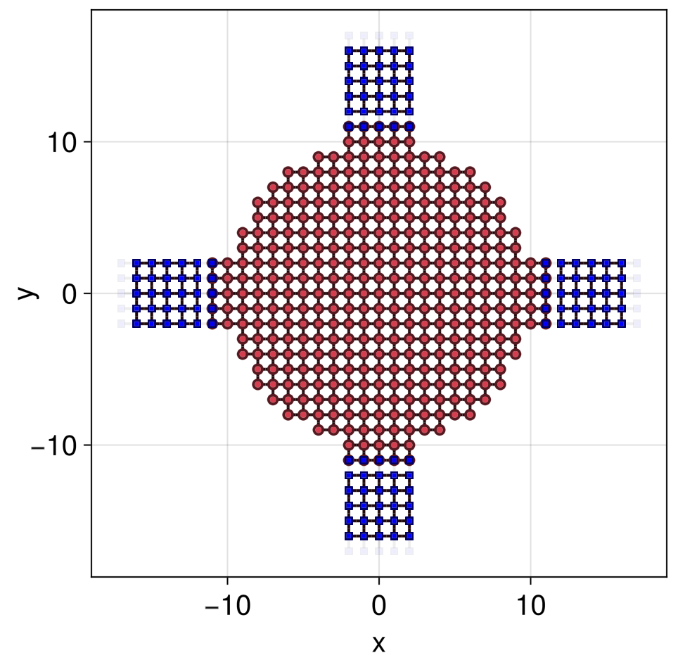
Note that since we did not specify the solver in greenfunction, the L=0 default GS.SparseLU() was taken.
We can also visualize glead, which is defined on a 1D lattice with a boundary. Boundary cells are shown by default in red
Its important un appreciate that a g::GreenFunction represents the retarded Green function between sites in a given AbstractHamiltonian, but not on sites of the coupled AbstractHamiltonians of its attached self-energies. Therefore, gcentral above cannot yield observables in the leads (blue sites above), only on the red sites. To obtain observables in a given lead, its GreenFunction must be constructed, with an attached self-energy coming from the central region plus the other three leads.
Slicing and evaluation
As explained above, a g::GreenFunction represents a Green function of an OpenHamiltonian (i.e. AbstractHamiltonian with zero or more self-energies), but it does so for any energy ω or lattice sites.
- To specify `ω` (plus any parameters `params` in the underlying `AbstractHamiltonian`) we use the syntax `g(ω; params...)`, which yields an `gω::GreenSolution`
- To specify source (`sⱼ`) and drain (`sᵢ`) sites we use the syntax `g[sᵢ, sⱼ]` or `g[sᵢ] == g[sᵢ,sᵢ]`, which yields a `gs::GreenSlice`. `sᵢ` and `sⱼ` can be `SiteSelectors(; sites...)`, or an integer denoting a specific contact (i.e. sites with an attached self-energy) or `:` denoting all contacts merged together.
- If we specify both of the above we get the Green function between the orbitals of the specified sites at the specified energy, in the form of an `OrbitalSliceMatrix`, which is a special `AbstractMatrix` that knows about the orbitals in the lattice over which its matrix elements are defined.
Let us see this in action using the example from the previous section
julia> g[1, 3]
GreenSlice{Float64,2,0}: Green function at arbitrary energy, but at a fixed lattice positions

julia> g(0.2)
GreenSolution{Float64,2,0}: Green function at arbitrary positions, but at a fixed energy

julia> g(0.2)[1, 3]
5×5 OrbitalSliceArray{ComplexF64,Array}:
 -2.56906+0.000123273im  -4.28767+0.00020578im   -4.88512+0.000234514im  -4.28534+0.00020578im    -2.5664+0.000123273im
 -4.28767+0.00020578im   -7.15613+0.00034351im   -8.15346+0.000391475im  -7.15257+0.00034351im    -4.2836+0.000205781im
 -4.88512+0.000234514im  -8.15346+0.000391475im  -9.29002+0.000446138im  -8.14982+0.000391476im  -4.88095+0.000234514im
 -4.28534+0.00020578im   -7.15257+0.00034351im   -8.14982+0.000391476im  -7.14974+0.000343511im  -4.28211+0.000205781im
  -2.5664+0.000123273im   -4.2836+0.000205781im  -4.88095+0.000234514im  -4.28211+0.000205781im  -2.56469+0.000123273im

julia> g(0.2)[siteselector(region = RP.circle(1, (0.5, 0))), 3]
2×5 OrbitalSliceArray{ComplexF64,Array}:
 0.0749214+3.15744e-8im   0.124325+5.27948e-8im   0.141366+6.01987e-8im   0.124325+5.27948e-8im  0.0749214+3.15744e-8im
-0.374862+2.15287e-5im -0.625946+3.5938e-5im -0.712983+4.09561e-5im -0.624747+3.59379e-5im -0.37348+2.15285e-5imIn the same way we can fix all parameters of a h::ParametricHamiltonian with h´=h(;params...) (which produces a h´::Hamiltonian without any parametric dependencies), we can similarly fix all parameters in a g::GreenFunction (or g::GreenSlice) with g(; params...), which produces a new GreenFunction (or GreenSlice). Note that, like in the case of h, this fixes all parameters. Any parameter that is not specify will be fixed to its default value.
Diagonal slices
There is a special form of slicing that requests just the diagonal of a given g[sᵢ] == g[sᵢ,sᵢ]. It uses the syntax g[diagonal(sᵢ)]. Let us see it in action in a multiorbital example in 2D
julia> g = HP.graphene(a0 = 1, t0 = 1, orbitals = 2) |> greenfunction
GreenFunction{Float64,2,2}: Green function of a Hamiltonian{Float64,2,2}
  Solver          : AppliedBandsGreenSolver
  Contacts        : 0
  Contact solvers : ()
  Contact sizes   : ()
  Hamiltonian{Float64,2,2}: Hamiltonian on a 2D Lattice in 2D space
    Bloch harmonics  : 5
    Harmonic size    : 2 × 2
    Orbitals         : [2, 2]
    Element type     : 2 × 2 blocks (ComplexF64)
    Onsites          : 0
    Hoppings         : 6
    Coordination     : 3.0

julia> g(0.5)[diagonal(cells = (0, 0))]
4×4 OrbitalSliceMatrix{ComplexF64,LinearAlgebra.Diagonal{ComplexF64, Vector{ComplexF64}}}:
 -0.349736-0.311836im        0.0+0.0im             0.0+0.0im             0.0+0.0im
       0.0+0.0im       -0.349736-0.311836im        0.0+0.0im             0.0+0.0im
       0.0+0.0im             0.0+0.0im       -0.349736-0.311836im        0.0+0.0im
       0.0+0.0im             0.0+0.0im             0.0+0.0im       -0.349736-0.311836im
Note that we get an OrbitalSliceVector, which is equal to the diagonal diag(g(0.5)[cells = (0, 0)]). Like the g OrbitalSliceMatrix, this vector is resolved in orbitals, of which there are two per site and four per unit cell in this case. Using diagonal(sᵢ; kernel = K) we can collect all the orbitals of different sites, and compute tr(g[site, site] * K) for a given matrix K. This is useful to obtain spectral densities. In the above example, and interpreting the two orbitals per site as the electron spin, we could obtain the spin density along the x axis, say, using σx = SA[0 1; 1 0] as kernel,
julia> g(0.5)[diagonal(cells = (0, 0), kernel = SA[0 1; 1 0])]
2×2 OrbitalSliceMatrix{ComplexF64,LinearAlgebra.Diagonal{ComplexF64, Vector{ComplexF64}}}:
 -2.57031e-12-2.62859e-17im          0.0+0.0im
          0.0+0.0im          2.57031e-12+2.27291e-17im
which is zero in this spin-degenerate case
An v::OrbitalSliceVector and m::OrbitalSliceMatrix are both a::OrbitalSliceArray, and wrap conventional arrays, with e.g. conventional axes. They also provide, however, orbaxes(a), which are a tuple of OrbitalSliceGrouped. These are LatticeSlices that represent orbitals grouped by sites. They allow an interesting additional functionality. You can index v[sitelector(...)] or m[rowsiteselector, colsiteselector] to obtain a new OrbitalSliceArray of the selected rows and cols. The full machinery of siteselector applies. One can also use a lower-level v[sites(cell_index, site_indices)] to obtain an unwrapped AbstractArray, without building new orbaxes. See OrbitalSliceArray for further details.
Visualizing a Green function
We can use qplot to visualize a GreenSolution in space. Here we define a bounded square lattice with an interesting shape, and attach a model self-energy to the right. Then we compute the Green function from each orbital in the contact to any other site in the lattice, and compute the norm over contact sites. The resulting vector is used as a shader for the color and radius of sites when plotting the system
julia> h = LP.square() |> onsite(4) - hopping(1) |> supercell(region = r -> norm(r) < 40*(1+0.2*cos(5*atan(r[2],r[1]))));

julia> g = h |> attach(@onsite(ω -> -im), region = r -> r[1] ≈ 47) |> greenfunction;

julia> gx1 = sum(abs2, g(0.1)[siteselector(), 1], dims = 2);

julia> qplot(h, hide = :hops, sitecolor = (i, r) -> gx1[i], siteradius = (i, r) -> gx1[i], minmaxsiteradius = (0, 2), sitecolormap = :balance)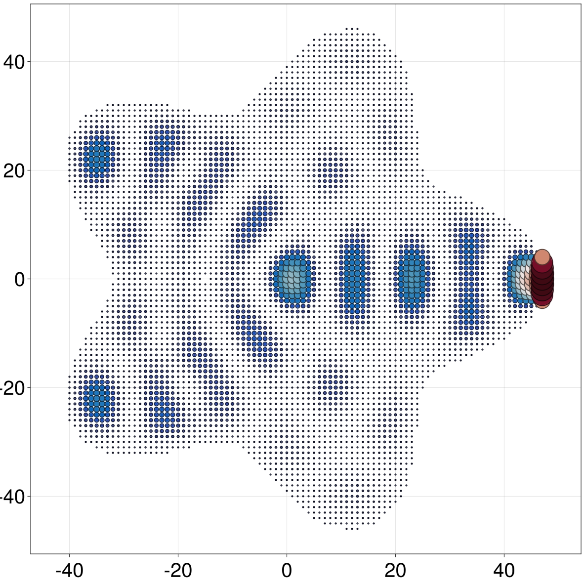
Since, currently, g(ω)[sᵢ, sⱼ] yields a Matrix over orbitals (instead of over sites), the above example requires single-orbital sites to work. In the future we will probably introduce a way to slice a GreenSolution over sites, similar to the way diagonal works. For the moment, one can use observables like ldos for visualization (see next section), which are all site-based by default.