Lattices

Constructing a Lattice from scratch

Consider a lattice like graphene's. It has two sublattices, A and B, forming a 2D honeycomb pattern in space. The position of site A and B inside the unitcell are [0, -a0/(2√3)] and [0, a0/(2√3)], respectively. The Bravais vectors are A₁, A₂ = a0 * [± cos(π/3), sin(π/3)]. If we set the lattice constant to a0 = √3 (so the carbon-carbon distance is 1), one way to build this lattice in Quantica.jl would be

julia> A₁, A₂ = √3 .* (cos(π/3), sin(π/3)),
                √3 .* (-cos(π/3), sin(π/3));

julia> sA, sB = sublat((0, -1/2), name = :A),
                sublat((0,  1/2), name = :B);

julia> lattice(sA, sB, bravais = (A₁, A₂))
Lattice{Float64,2,2} : 2D lattice in 2D space
  Bravais vectors : [[0.866025, 1.5], [-0.866025, 1.5]]
  Sublattices     : 2
    Names         : (:A, :B)
    Sites         : (1, 1) --> 2 total per unit cell

Tuple, SVector and SMatrix

Note that we have used Tuples, such as (0, 1/2) instead of Vectors, like [0, 1/2]. In Julia small-length Tuples are much more efficient as containers than Vectors, since their length is known and fixed at compile time. Static vectors (SVector) and matrices (SMatrix) are also available to Quantica, which are just as efficient as Tuples, and they also implement linear algebra operations. They may be entered as e.g. SA[0, 1/2] and SA[1 0; 0 1], respectively. For efficiency, always use Tuple, SVector and SMatrix in Quantica.jl where possible.

If we don't plan to address the two sublattices individually, we could also fuse them into one, like

julia> lat = lattice(sublat((0, 1/2), (0, -1/2)), bravais = (A₁, A₂))
Lattice{Float64,2,2} : 2D lattice in 2D space
  Bravais vectors : [[0.866025, 1.5], [-0.866025, 1.5]]
  Sublattices     : 1
    Names         : (:A,)
    Sites         : (2,) --> 2 total per unit cell

This lattice has type Lattice{T,E,L}, with T = Float64 the numeric type of position coordinates, E = 2 the dimension of embedding space, and L = 2 the number of Bravais vectors (i.e. the lattice dimension). Both T and E, and even the Sublat names can be overridden when creating a lattice. One can also provide the Bravais vectors as a matrix, with each Aᵢ as a column.

julia> Amat = √3 * SA[-cos(π/3) cos(π/3); sin(π/3) sin(π/3)];

julia> lat´ = lattice(sA, sB, bravais = Amat, type = Float32, dim = 3, names = (:C, :D))
Lattice{Float32,3,2} : 2D lattice in 3D space
  Bravais vectors : Vector{Float32}[[-0.866025, 1.5, 0.0], [0.866025, 1.5, 0.0]]
  Sublattices     : 2
    Names         : (:C, :D)
    Sites         : (1, 1) --> 2 total per unit cell

Advanced: `dim = Val(E)` vs. `dim = E`

For the dim keyword above we can alternatively use dim = Val(3), which is slightly more efficient, because the value is encoded as a type. This is a "Julia thing" (related to the concept of type stability), and can be ignored upon a first contact with Quantica.jl.

One can also convert an existing lattice like the above to have a different type, embedding dimension, Bravais vectors and Sublat names with lattice(lat; kw...). For example

julia> lat´´ = lattice(lat´, type = Float16, dim = 2, names = (:Boron, :Nitrogen))
Lattice{Float16,2,2} : 2D lattice in 2D space
  Bravais vectors : Vector{Float16}[[-0.866, 1.5], [0.866, 1.5]]
  Sublattices     : 2
    Names         : (:Boron, :Nitrogen)
    Sites         : (1, 1) --> 2 total per unit cell

A list of site positions in a lattice lat can be obtained with sites(lat), or sites(lat, sublat) to restrict to a specific sublattice

julia> sites(lat´´)
2-element Vector{SVector{2, Float16}}:
 [0.0, -0.5]
 [0.0, 0.5]

julia> sites(lat´´, :Nitrogen)
1-element view(::Vector{SVector{2, Float16}}, 2:2) with eltype SVector{2, Float16}:
 [0.0, 0.5]

Similarly, the Bravais matrix of a lat can be obtained with bravais_matrix(lat).

Lattice presets

Quantica.jl provides a range of presets. A preset is a pre-built object of some type. In particular we have Lattice presets, defined in the submodule LatticePresets (also called LP for convenience), that include a number of classical lattices in different dimensions:

LP.linear: linear 1D lattice
LP.square: square 2D lattice
LP.honeycomb: honeycomb 2D lattice
LP.cubic: cubic 3D lattice
LP.bcc: body-centered cubic 3D lattice
LP.fcc: face-centered cubic 3D lattice

To obtain a lattice from a preset one simply calls it, e.g. LP.honecyomb(; kw...). One can modify any of these LatticePresets by passing a bravais, type, dim or names keyword. One can also use a new keyword a0 for the lattice constant (a0 = 1 by default). The lattice lat´´ above can thus be also obtained with

julia> lat´´ = LP.honeycomb(a0 = √3, type = Float16, names = (:Boron, :Nitrogen))
Lattice{Float16,2,2} : 2D lattice in 2D space
  Bravais vectors : Vector{Float16}[[0.866, 1.5], [-0.866, 1.5]]
  Sublattices     : 2
    Names         : (:Boron, :Nitrogen)
    Sites         : (1, 1) --> 2 total per unit cell

Quantica's Presets library

Quantica comes with four submodules that provide different kinds of presets: LatticePresets (LP), HamiltonianPresets (HP), RegionPresets (RP) and ExternalPresets (EP). LP provides a collection of standard lattices, HP some premade model Hamiltonians such as HP.graphene or HP.twisted_bilayer_graphene, RP some geometric regions such as RP.circle or RP.cuboid, and EP some importers of externally produced objects such as EP.wannier90 to import Wannier90 files (see Advanced for details on the latter). This library of presets is expected to grow with time. The docstring for the submodule or the preset function can be queried for a description of the available options.

Visualization

To produce an interactive visualization of Lattices or other Quantica.jl object you need to load GLMakie.jl, CairoMakie.jl or some other plotting backend from the Makie repository (i.e. do using GLMakie, see also Installation). Then, a number of new plotting functions will become available. The main one is qplot. A Lattice is represented, by default, as the sites in a unitcell plus the Bravais vectors.

julia> using GLMakie

julia> lat = LP.honeycomb()

julia> qplot(lat, hide = nothing)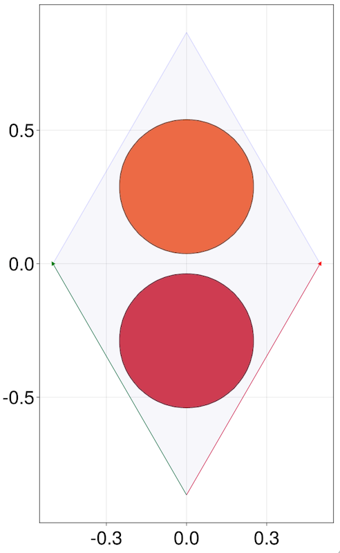

qplot accepts a large number of keywords to customize your plot. In the case of lattice, most of these are passed over to the function plotlattice, specific to Lattices and Hamiltonians. In the case above, hide = nothing means "don't hide any element of the plot". See the qplot and plotlattice docstrings for details.

GLMakie.jl vs CairoMakie.jl

GLMakie.jl is optimized for interactive GPU-accelerated, rasterized plots. If you need to export to PDF for publications or display plots inside a Jupyter notebook, use CairoMakie.jl instead, which in general renders non-interactive, but vector-based plots.

User-defined defaults for `qplot`

The command qplotdefaults(; axis, figure) can be used to define the default value of figure and axis keyword arguments of qplot. Example: to fix the size of all subsequent plots, do qplotdefaults(; figure = (size = (1000, 1000),)).

SiteSelectors

A central concept in Quantica.jl is that of a "selector". There are two types of selectors, SiteSelectors and HopSelectors. SiteSelectors are a set of directives or rules that define a subset of its sites. SiteSelector rules are defined through three keywords:

region: a boolean function of allowed site positions r.
sublats: allowed sublattices of selected sites
cells: allowed cell indices of selected sites

Similarly, HopSelectors can be used to select a number of site pairs, and will be used later to define hoppings in tight-binding models (see further below).

As an example, let us define a SiteSelector that picks all sites belonging to the :B sublattice of a given lattice within a circle of radius 10

julia> s = siteselector(region = r -> norm(r) <= 10, sublats = :B)
SiteSelector: a rule that defines a finite collection of sites in a lattice
  Region            : Function
  Sublattices       : B
  Cells             : any

Note that this selector is defined independently of the lattice. To apply it to a lattice lat we do lat[s], which results in a LatticeSlice (i.e. a finite portion, or slice, of lat)

julia> lat = LP.honeycomb(); lat[s]
LatticeSlice{Float64,2,2} : collection of subcells for a 2D lattice in 2D space
  Cells       : 363
  Cell range  : ([-11, -11], [11, 11])
  Total sites : 363

The Cell range above are the corners of a bounding box in cell-index space that contains all unit cell indices with at least one selected site.

Let's plot it

julia> qplot(lat[s], hide = ())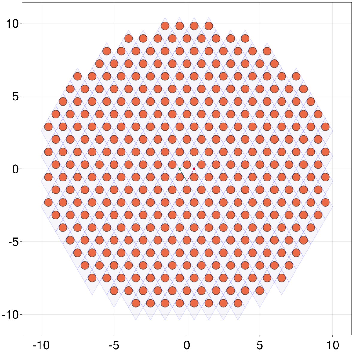

qplot selector

The above qplot(lat[s]) can also be written as qplot(lat, selector = s), which will be useful when plotting AbstractHamiltonians.

Sites of a LatticeSlice

Collect the site positions of a LatticeSlice into a vector with collect(sites(ls)). If you do sites(ls) instead, you will get a lazy generator that can be used to iterate efficiently among site positions without allocating them in memory.

Apart from region and sublats we can also restrict the unitcells by their cell index. For example, to select all sites in unit cells within the above bounding box we can do

julia> s´ = siteselector(cells = CartesianIndices((-11:11, -11:11)))
SiteSelector: a rule that defines a finite collection of sites in a lattice
  Region            : any
  Sublattices       : any
  Cells             : CartesianIndices((-11:11, -11:11))

julia> lat[s´]
LatticeSlice{Float64,2,2} : collection of subcells for a 2D lattice in 2D space
  Cells       : 529
  Cell range  : ([-11, -11], [11, 11])
  Total sites : 1058

We can often omit constructing the SiteSelector altogether by using the keywords directly

julia> ls = lat[cells = n -> 0 <= n[1] <= 2 && abs(n[2]) < 3, sublats = :A]
LatticeSlice{Float64,2,2} : collection of subcells for a 2D lattice in 2D space
  Cells       : 15
  Cell range  : ([0, -2], [2, 2])
  Total sites : 15

Selectors are very expressive and powerful. Do check siteselector and hopselector docstrings for more details.

Transforming lattices

We can transform lattices using supercell, reverse, transform, translate.

As a periodic structure, the choice of the unitcell in an unbounded lattice is, to an extent, arbitrary. Given a lattice lat we can obtain another with a unit cell 3 times larger with supercell(lat, 3)

julia> lat = supercell(LP.honeycomb(), 3)
Lattice{Float64,2,2} : 2D lattice in 2D space
  Bravais vectors : [[1.5, 2.598076], [-1.5, 2.598076]]
  Sublattices     : 2
    Names         : (:A, :B)
    Sites         : (9, 9) --> 18 total per unit cell

More generally, given a lattice lat with Bravais matrix Amat = bravais_matrix(lat), we can obtain a larger one with Bravais matrix Amat´ = Amat * S, where S is a square matrix of integers. In the example above, S = SA[3 0; 0 3]. The columns of S represent the coordinates of the new Bravais vectors in the basis of the old Bravais vectors. A more general example with e.g. S = SA[3 1; -1 2] can be written either in terms of S or of its columns

julia> supercell(lat, SA[3 1; -1 2]) == supercell(lat, (3, -1), (1, 2))
true

We can also use supercell to reduce the number of Bravais vectors, and hence the lattice dimensionality. To construct a new lattice with a single Bravais vector A₁´ = 3A₁ - A₂, just omit the second one

julia> supercell(lat, (3, -1))
Lattice{Float64,2,1} : 1D lattice in 2D space
  Bravais vectors : [[6.0, 5.196152]]
  Sublattices     : 2
    Names         : (:A, :B)
    Sites         : (27, 27) --> 54 total per unit cell

Its important to note that the lattice will be bounded along directions different from the specified Bravais vectors. With the syntax above, the new unitcell will be minimal. We may however define how many sites to include in the new unitcell by adding a SiteSelector directive to be applied in the non-periodic directions. For example, to create a 10 * a0 wide, honeycomb nanoribbon we can do

julia> lat = supercell(LP.honeycomb(), (1,-1), region = r -> -5 <= r[2] <= 5)
Lattice{Float64,2,1} : 1D lattice in 2D space
  Bravais vectors : [[1.0, 0.0]]
  Sublattices     : 2
    Names         : (:A, :B)
    Sites         : (12, 12) --> 24 total per unit cell

julia> qplot(lat[cells = -7:7])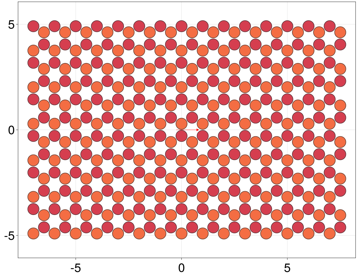

No need to build selectors explicitly

Note that we we didn't build a siteselector(region = ...) object to pass it to supercell. Instead, as shown above, we passed the corresponding keywords directly to supercell, which then takes care to build the selector internally.

To simply reverse the direction of the Bravais vectors of a lattice, while leaving the site positions unchanged, use reverse (or reverse! to do it in-place)

julia> reverse(LP.square())
Lattice{Float64,2,2} : 2D lattice in 2D space
  Bravais vectors : [[-1.0, -0.0], [-0.0, -1.0]]
  Sublattices     : 1
    Names         : (:A,)
    Sites         : (1,) --> 1 total per unit cell

To transform a lattice, so that site positions r become f(r) use transform

julia> f(r) = SA[0 1; 1 0] * r
f (generic function with 1 method)

julia> rotated_honeycomb = transform(LP.honeycomb(a0 = √3), f)
Lattice{Float64,2,2} : 2D lattice in 2D space
  Bravais vectors : [[1.5, 0.866025], [1.5, -0.866025]]
  Sublattices     : 2
    Names         : (:A, :B)
    Sites         : (1, 1) --> 2 total per unit cell

julia> sites(rotated_honeycomb)
2-element Vector{SVector{2, Float64}}:
 [-0.5, 0.0]
 [0.5, 0.0]

To translate a lattice by a displacement vector δr use translate

julia> δr = SA[0, 1];

julia> sites(translate(rotated_honeycomb, δr))
2-element Vector{SVector{2, Float64}}:
 [-0.5, 1.0]
 [0.5, 1.0]

Currying: chaining transformations with the `|>` operator

Many functions in Quantica.jl have a "curried" version that allows them to be chained together using the pipe operator |>.

Definition of currying

The curried version of a function f(x1, x2...) is f´ = x1 -> f(x2...), so that the curried form of f(x1, x2...) is x2 |> f´(x2...), or f´(x2...)(x1). This gives the first argument x1 a privileged role. Users of object-oriented languages such as Python may find this use of the |> operator somewhat similar to the way the dot operator works there (i.e. x1.f(x2...)).

The last example above can then be written as

julia> LP.honeycomb(a0 = √3) |> transform(f) |> translate(δr) |> sites
2-element Vector{SVector{2, Float64}}:
 [-0.5, 1.0]
 [0.5, 1.0]

This type of curried syntax is natural in Quantica, and will be used extensively in this tutorial.