Hamiltonians
We build a Hamiltonian by combining a Lattice and a TightbindingModel, optionally specifying also the number of orbitals on each sublattice if there is more than one. A spinful graphene model (two orbitals per site in both sublattices) with nearest neighbor hopping t0 = 2.7 would be written as
julia> lat = LP.honeycomb(); model = hopping(2.7*I);

julia> h = hamiltonian(lat, model; orbitals = 2)
Hamiltonian{Float64,2,2}: Hamiltonian on a 2D Lattice in 2D space
  Bloch harmonics  : 5
  Harmonic size    : 2 × 2
  Orbitals         : [2, 2]
  Element type     : 2 × 2 blocks (ComplexF64)
  Onsites          : 0
  Hoppings         : 6
  Coordination     : 3.0
A crucial thing to remember when defining multi-orbital Hamiltonians as the above is that onsite and hopping amplitudes need to be matrices of the correct size. The symbol I in Julia represents the identity matrix of any size, which is convenient to define a spin-preserving hopping in the case above. An alternative would be to use model = hopping(2.7*SA[1 0; 0 1]).
Non-homogeneous multiorbital models are more advanced but are fully supported in Quantica.jl. Just use orbitals = (n₁, n₂,...) to have nᵢ orbitals in sublattice i, and make sure your model is consistent with that. As in the case of the dim keyword in lattice, you can also use Val(nᵢ) for marginally faster construction.
Similarly to LatticePresets, we also have HamiltonianPresets, also aliased as HP. Currently, we have only HP.graphene(...) and HP.twisted_bilayer_graphene(...), but we expect to extend this library in the future (see the docstring of HP).
A more elaborate example: the Kane-Mele model
The Kane-Mele model for graphene describes intrinsic spin-orbit coupling (SOC), in the form of an imaginary second-nearest-neighbor hopping between same-sublattice sites, with a sign that alternates depending on hop direction dr. A possible implementation in Quantica.jl would be
SOC(dr) = 0.05 * ifelse(iseven(round(Int, atan(dr[2], dr[1])/(pi/3))), im, -im)

model =
  hopping(1, range = neighbors(1)) +
  hopping((r, dr) ->  SOC(dr); sublats = :A => :A, range = neighbors(2)) +
  hopping((r, dr) -> -SOC(dr); sublats = :B => :B, range = neighbors(2))

h = LatticePresets.honeycomb() |> model

qplot(h)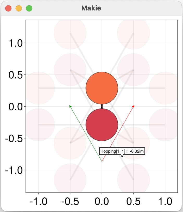
Interactive tooltips in the visualization of h are enabled by default (use keyword inspector = false to disable them). They allows to navigate each onsite and hopping amplitude graphically. Note that sites connected to the unit cell of h by some hopping are included, but are rendered with partial transparency by default.
ParametricHamiltonians
If we use a ParametricModel instead of a simple TightBindingModel we will obtain a ParametricHamiltonian instead of a simple Hamiltonian, both of which are subtypes of the AbstractHamiltonian type
julia> model_param = @hopping((; t = 2.7) -> t*I);

julia> h_param = hamiltonian(lat, model_param; orbitals = 2)
ParametricHamiltonian{Float64,2,2}: Parametric Hamiltonian on a 2D Lattice in 2D space
  Bloch harmonics  : 5
  Harmonic size    : 2 × 2
  Orbitals         : [2, 2]
  Element type     : 2 × 2 blocks (ComplexF64)
  Onsites          : 0
  Hoppings         : 6
  Coordination     : 3.0
  Parameters       : [:t]
We can also apply Modifiers by passing them as extra arguments to hamiltonian, which results again in a ParametricHamiltonian with the parametric modifiers applied
julia> peierls! = @hopping!((t, r, dr; Bz = 0) -> t * cis(-Bz/2 * SA[-r[2], r[1]]' * dr));

julia> h_param_mod = hamiltonian(lat, model_param, peierls!; orbitals = 2)
ParametricHamiltonian{Float64,2,2}: Parametric Hamiltonian on a 2D Lattice in 2D space
  Bloch harmonics  : 5
  Harmonic size    : 2 × 2
  Orbitals         : [2, 2]
  Element type     : 2 × 2 blocks (ComplexF64)
  Onsites          : 0
  Hoppings         : 6
  Coordination     : 3.0
  Parameters       : [:Bz, :t]
Note that SA[-r[2], r[1]] above is a 2D SVector, because since the embedding dimension is E = 2, both r and dr are also 2D SVectors.
We can also apply modifiers to an already constructed AbstractHamiltonian. The following is equivalent to the above
julia> h_param_mod = hamiltonian(h_param, peierls!);We can add as many modifiers as we need by passing them as extra arguments to hamiltonian, and they will be applied sequentially, one by one. Beware, however, that modifiers do not necessarily commute, in the sense that the result will in general depend on their order.
We can obtain a plain Hamiltonian from a ParametricHamiltonian by applying specific values to its parameters. To do so, simply use the call syntax with parameters as keyword arguments
julia> h_param_mod(Bz = 0.1, t = 1)
Hamiltonian{Float64,2,2}: Hamiltonian on a 2D Lattice in 2D space
  Bloch harmonics  : 5
  Harmonic size    : 2 × 2
  Orbitals         : [2, 2]
  Element type     : 2 × 2 blocks (ComplexF64)
  Onsites          : 0
  Hoppings         : 6
Coordination : 3.0The common cases lat |> hamiltonian(model) (or hamiltonian(lat, model)) and h |> hamiltonian(modifier) (or hamiltonian(h, modifier)) can be also written as lat |> model and h |> modifier, respectively. Hence hamiltonian(lat, model, modifier) may be written as lat |> model |> modifier. This form however does not allow to specify the number of orbitals per sublattice (it will be one, the default).
Obtaining actual matrices
For an L-dimensional h::AbstractHamiltonian (i.e. defined on a Lattice with L Bravais vectors), the Hamiltonian matrix between any unit cell with cell index n and another unit cell at n+dn (here known as a Hamiltonian "harmonic") is given by h[dn]
julia> h[(1,0)]
4×4 SparseArrays.SparseMatrixCSC{ComplexF64, Int64} with 4 stored entries:
     ⋅          ⋅      2.7+0.0im  0.0+0.0im
     ⋅          ⋅      0.0+0.0im  2.7+0.0im
     ⋅          ⋅          ⋅          ⋅
     ⋅          ⋅          ⋅          ⋅

julia> h[(0,0)]
4×4 SparseArrays.SparseMatrixCSC{ComplexF64, Int64} with 8 stored entries:
     ⋅          ⋅      2.7+0.0im  0.0+0.0im
     ⋅          ⋅      0.0+0.0im  2.7+0.0im
 2.7+0.0im  0.0+0.0im      ⋅          ⋅
0.0+0.0im 2.7+0.0im ⋅ ⋅We can use Tuples or SVectors for cell distance indices dn. An empty Tuple dn = () will always return the main intra-unitcell harmonic: h[()] = h[(0,0...)] = h[SA[0,0...]].
If the Hamiltonian has a bounded lattice (i.e. it has L=0 Bravais vectors), we will simply use an empty tuple to obtain its matrix h[()]. This is not in conflict with the above syntax.
Note that if h is a ParametricHamiltonian, such as h_param above, we will get zeros in place of the unspecified parametric terms, unless we actually first specify the values of the parameters
julia> h_param[(0,0)] # Parameter t is not specified -> it is not applied
4×4 SparseArrays.SparseMatrixCSC{ComplexF64, Int64} with 8 stored entries:
     ⋅          ⋅      0.0+0.0im  0.0+0.0im
     ⋅          ⋅      0.0+0.0im  0.0+0.0im
 0.0+0.0im  0.0+0.0im      ⋅          ⋅
 0.0+0.0im  0.0+0.0im      ⋅          ⋅

julia> h_param(t=2)[(0,0)]
4×4 SparseArrays.SparseMatrixCSC{ComplexF64, Int64} with 8 stored entries:
     ⋅          ⋅      2.0+0.0im  0.0+0.0im
     ⋅          ⋅      0.0+0.0im  2.0+0.0im
 2.0+0.0im  0.0+0.0im      ⋅          ⋅
0.0+0.0im 2.0+0.0im ⋅ ⋅The above behavior for unspecified parameters is not set in stone and may change in future versions. Another option would be to apply their default values (which may, however, not exist).
We are usually not interested in the harmonics h[dn] themselves, but rather in the Bloch matrix of a Hamiltonian
$H(\phi) = \sum_{dn} H_{dn} \exp(-i \phi * dn)$
where $H_{dn}$ are the Hamiltonian harmonics, $\phi = (\phi_1, \phi_2...) = (k\cdot A_1, k\cdot A_2...)$ are the Bloch phases, $k$ is the Bloch wavevector and $A_i$ are the Bravais vectors.
We obtain the Bloch matrix using the syntax h(ϕ; params...)
julia> h((0,0))
4×4 SparseArrays.SparseMatrixCSC{ComplexF64, Int64} with 8 stored entries:
     ⋅          ⋅      8.1+0.0im  0.0+0.0im
     ⋅          ⋅      0.0+0.0im  8.1+0.0im
 8.1+0.0im  0.0+0.0im      ⋅          ⋅
 0.0+0.0im  8.1+0.0im      ⋅          ⋅

julia> h_param_mod((0.2, 0.3); B = 0.1)
4×4 SparseArrays.SparseMatrixCSC{ComplexF64, Int64} with 8 stored entries:
         ⋅                  ⋅          7.92559-1.33431im      0.0+0.0im
         ⋅                  ⋅              0.0+0.0im      7.92559-1.33431im
 7.92559+1.33431im      0.0+0.0im              ⋅                  ⋅
     0.0+0.0im      7.92559+1.33431im          ⋅                  ⋅
Note that unspecified parameters take their default values when using the call syntax (as per the standard Julia convention). Any unspecified parameter that does not have a default value will produce an UndefKeywordError error.
Transforming Hamiltonians
Like with lattices, we can transform an h::AbstractHamiltonians using supercell, reverse, transform and translate. All these except supercell operate only on the underlying lattice(h) of h, leaving the hoppings and onsite elements unchanged. Meanwhile, supercell acts on lattice(h) but also copies the hoppings and onsites of h onto the new sites, preserving the periodicity of the original h.
Additionally, we can also use stitch and @stitch, which makes the h lattice periodic along some (or all) of its Bravais vectors, while leaving the rest unbounded.
julia> stitch(HP.graphene(), (0, :))
Hamiltonian{Float64,2,1}: Hamiltonian on a 1D Lattice in 2D space
  Bloch harmonics  : 3
  Harmonic size    : 2 × 2
  Orbitals         : [1, 1]
  Element type     : scalar (ComplexF64)
  Onsites          : 0
  Hoppings         : 4
  Coordination     : 2.0
The phases argument of stitch(h, phases) is a Tuple of real numbers and/or colons (:), of length equal to the lattice dimension of h. Each real number ϕᵢ corresponds to a Bravais vector along which the transformed lattice will become periodic, picking up a phase exp(iϕᵢ) in the new hoppings, while each colon leaves the lattice unbounded along the corresponding Bravais vector. (Check the stitch and @stitch docstrings for additional syntax and functionality.) In a way, stitch is the dual to supercell, in that it applies a different boundary condition to the lattice along the eliminated Bravais vectors, periodic instead of open, as in the case of supercell. The phases ϕᵢ are also connected to Bloch phases, in the sense that e.g. stitch(h, (ϕ₁, :))(; ϕ₂) == h(ϕ₁, ϕ₂).
It's important to understand that, when transforming an h::AbstractHamiltonian, the model used to build h is not re-evaluated. Hoppings and onsite energies are merely copied so as to preserve the periodicity of the original h. As a consequence, these two constructions give different Hamiltonians
julia> h1 = LP.linear() |> supercell(4) |> hamiltonian(onsite(r -> r[1]));

julia> h2 = LP.linear() |> hamiltonian(onsite(r -> r[1])) |> supercell(4);
In the case of h1 the onsite model is applied to the 4-site unitcell. Since each site has a different position, each gets a different onsite energy.
julia> h1[()]
4×4 SparseArrays.SparseMatrixCSC{ComplexF64, Int64} with 4 stored entries:
 0.0+0.0im      ⋅          ⋅          ⋅
     ⋅      1.0+0.0im      ⋅          ⋅
     ⋅          ⋅      2.0+0.0im      ⋅
     ⋅          ⋅          ⋅      3.0+0.0im
In contrast h2 first gets the onsite model applied with a 1-site unitcell at position r = SA[0], so all sites in the lattice get onsite energy zero. Only then it is expanded with supercell, which generates a 4-site unitcell with zero onsite energy on all its sites
julia> h2[()]
4×4 SparseArrays.SparseMatrixCSC{ComplexF64, Int64} with 4 stored entries:
 0.0+0.0im      ⋅          ⋅          ⋅
     ⋅      0.0+0.0im      ⋅          ⋅
     ⋅          ⋅      0.0+0.0im      ⋅
     ⋅          ⋅          ⋅      0.0+0.0im
As a consequence, h and supercell(h) represent exactly the same system, with the same observables, but with a different choice of unitcell.
These two different behaviors make sense in different situations, so it is important to be aware of the order dependence of transformations. Similar considerations apply to transform, translate and stitch when models are position dependent.
Combining Hamiltonians
Multiple h::AbstractHamiltonians (or multiple l::Lattices) can be combined into one with combine.
julia> h1 = LP.linear(dim = 2) |> hopping(1); h2 = LP.linear(dim = 2, names = :B) |> hopping(1) |> translate(SA[0,1]) |> @onsite!((o; p=1) -> o+p);

julia> combine(h1, h2; coupling = hopping(2))
ParametricHamiltonian{Float64,2,1}: Parametric Hamiltonian on a 1D Lattice in 2D space
  Bloch harmonics  : 3
  Harmonic size    : 2 × 2
  Orbitals         : [1, 1]
  Element type     : scalar (ComplexF64)
  Onsites          : 0
  Hoppings         : 6
  Coordination     : 3.0
  Parameters       : [:p]
The coupling keyword, available when combining h::AbstractHamiltonians, is a hopping model that is applied between each h. It can be constrained as usual with hopselectors and also be parametric. If either coupling or any of the combined h is parametric, the result of combine will be a ParametricHamiltonian, or a Hamiltonian otherwise.
The objects to be combined must satisfy some conditions:
- They must have the same Bravais vectors (modulo reorderings), which will be then inherited by the combined object.
- Their embedding dimension must be the same
- They must have the same position type (the
TinAbstractHamiltonian{T}andLattice{T})